If you’ve ever searched for PID loop explained in simple terms, you’re in the right place.
Whether you’re a mechatronics student, a control systems engineer, or an automation professional — understanding the PID loop is one of the most essential skills you can develop. It powers thermostats, drone flight controllers, industrial robots, cruise control systems, and virtually every automated process that needs to stay on target.
In this guide, we’ll explain the PID loop from the ground up:
👉 What a PID loop is, how each term works, the math behind it, tuning methods, real-world applications, common problems, and a working Matlab implementation — all in one place.
Table of Contents
- What Is a PID Loop?
- How a PID Loop Works — The Closed-Loop System
- The Three Terms of a PID Loop Explained
- The PID Loop Equation
- Effects of Each Gain — Summary Table
- PID Loop Variants: P, PI, PD, PID
- How to Tune a PID Loop
- Real-World Applications of PID Loops
- Common PID Loop Problems and Fixes
- PID Loop in Code — Python Example
- Limitations of the PID Loop
- FAQ — PID Loop Explained
What Is a PID Loop?
A PID loop (Proportional-Integral-Derivative loop) is a closed-loop feedback control algorithm that continuously measures the difference between a desired target value and an actual measured value — called the error — and applies a calculated corrective output to drive that error toward zero.
The term “loop” refers to the continuous feedback cycle: measure → calculate → correct → measure again.
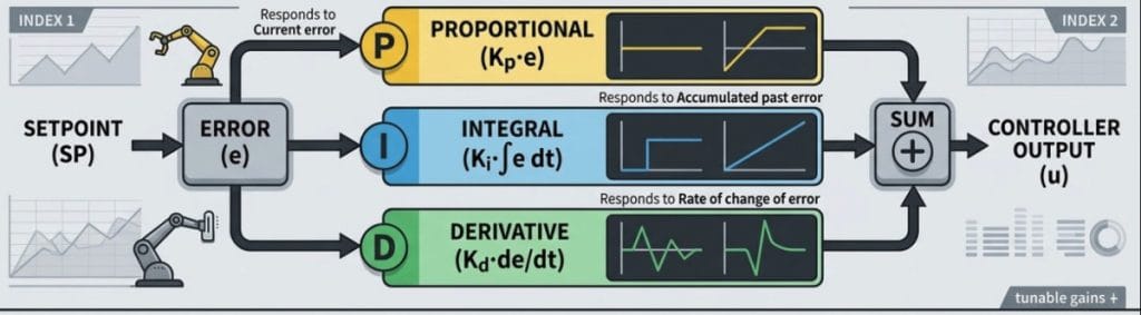
| Term | Stands For | What It Responds To |
|---|---|---|
| P | Proportional | Current error (right now) |
| I | Integral | Accumulated past error (history) |
| D | Derivative | Rate of change of error (near future) |
The controller output is the weighted sum of all three terms, each scaled by a tunable gain constant: Kp, Ki, and Kd.
🏛️ Historical Note: The mathematical foundation of the PID loop was first formalized by Russian-American engineer Nicolas Minorsky in 1922, while developing automatic ship steering for the U.S. Navy. He observed that expert helmsmen corrected course based on the current heading error, accumulated past drift, and the rate at which the error was changing — precisely the logic of P, I, and D.
How a PID Loop Works — The Closed-Loop System
To understand the PID loop, you first need to understand the closed-loop feedback system it lives inside.
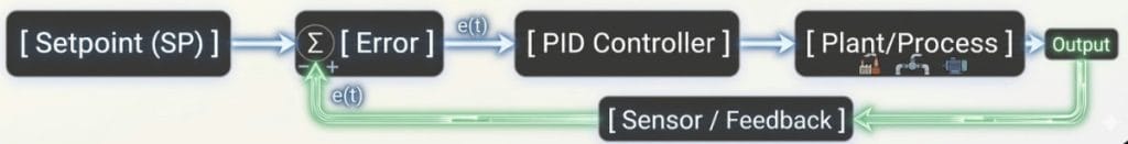
| Component | Role in the PID Loop |
|---|---|
| Setpoint (SP) | The desired target value (e.g., 100°C, 1500 RPM, 5V) |
| Process Variable (PV) | The actual measured value from the sensor |
| Error e(t) | e(t) = SP − PV — the gap the PID loop must close |
| Controller Output u(t) | The corrective signal sent to the actuator |
| Plant | The physical system being controlled (motor, heater, valve, etc.) |
| Feedback | Sensor reading continuously fed back to the controller |
The PID loop runs this cycle repeatedly — typically hundreds or thousands of times per second in embedded systems — constantly recalculating the error and adjusting the output.
The Three Terms of a PID Loop Explained
1. Proportional (P) — React to the Present Error
The proportional term produces an output directly proportional to the current error.
What it does: The larger the error, the larger the corrective action. If the temperature is 20°C below the setpoint, the heater fires at full power. As the temperature rises and the error shrinks, the heater power proportionally reduces.
The fundamental problem: Proportional control alone almost always results in a steady-state error (offset). As the system approaches the setpoint, the error — and therefore the corrective force — keeps shrinking. The system settles near the target, but rarely at it.
| Kp Too Low | Kp Optimal | Kp Too High |
|---|---|---|
| Sluggish response, large offset | Fast, stable response, small offset | Oscillation, potential instability |
2. Integral (I) — Correct the Accumulated Past Error
The integral term sums up the error over time and applies a correction proportional to the total accumulated error.
What it does: Even a tiny persistent error will cause the integral to keep growing, continuously pushing the output harder until the error is completely eliminated. This is how the integral term removes steady-state offset — the defining weakness of pure P control.
The catch — Integral Windup: If the system is far from its setpoint for an extended period (e.g., during a cold startup), the integral accumulates an excessively large value. When the setpoint is finally approached, this “wound-up” integral causes significant overshoot. Anti-windup strategies are essential in real implementations.
| Ki Too Low | Ki Optimal | Ki Too High |
|---|---|---|
| Slow elimination of offset | Clean, steady-state error = 0 | Overshoot, oscillation, windup |
3. Derivative (D) — Predict and Dampen
The derivative term reacts to the rate of change of the error — it predicts where the error is heading and applies a pre-emptive dampening correction.
What it does: If the error is collapsing rapidly (the system is approaching the setpoint fast), the derivative applies a “braking” force to prevent overshoot. It acts like a shock absorber — the faster the change, the harder it resists.
The catch — Noise Amplification: Differentiation amplifies high-frequency noise. Any electrical noise in the sensor signal gets magnified by the derivative term, producing erratic controller behavior. In practice, a low-pass filter is almost always applied to the derivative channel. Many engineers also apply the derivative to the process variable (not the error) to avoid derivative kick — the sudden spike in output when the setpoint changes instantaneously.
| Kd Too Low | Kd Optimal | Kd Too High |
|---|---|---|
| Overshoot, slow settling | Smooth approach, minimal overshoot | Noise amplification, instability |
The PID Loop Equation
The complete continuous-time PID loop equation is:
Where:
u(t)= controller output (the corrective action)e(t)= SP − PV (current error)Kp= proportional gainKi= integral gainKd= derivative gain
Discrete-Time Form (Embedded / Digital Systems)
In microcontrollers, PLCs, and digital systems, the PID loop runs in discrete time steps:
Where is the sampling period and k is the current time step index.
Effects of Each Gain — Summary Table
| Parameter | Rise Time | Overshoot | Settling Time | Steady-State Error | Stability |
|---|---|---|---|---|---|
| ↑ Kp | Decrease | Increase | Small change | Decrease | Degrade |
| ↑ Ki | Decrease | Increase | Increase | Eliminate | Degrade |
| ↑ Kd | Small change | Decrease | Decrease | No effect | Improve (if moderate) |
PID Loop Variants: P, PI, PD, PID
Not every application requires all three terms. Understanding when to simplify the PID loop is just as important as knowing how to tune the full version.
| Loop Type | Active Terms | Best Used When |
|---|---|---|
| P only | Kp | Fast systems where small offset is acceptable |
| PI | Kp + Ki | Most industrial processes — eliminates steady-state error without derivative noise issues |
| PD | Kp + Kd | Fast systems needing damping but where offset is acceptable |
| PID | Kp + Ki + Kd | Full control — where both precision and speed are required |
💡 Engineering Reality: The PI configuration is the most commonly deployed variant in industry. The derivative term is added only when the process has significant lag or oscillatory tendencies — because noise sensitivity makes D tricky to implement reliably in the field.
How to Tune a PID Loop
Tuning a PID loop means finding the right Kp, Ki, Kd values for your specific system. Here are the most widely used methods:
Method 1: Manual Tuning (Trial and Error)
The most hands-on approach to PID loop tuning:
- Set Ki = 0 and Kd = 0
- Increase Kp until the system responds well but just starts to oscillate
- Back off Kp slightly (about 50% of the oscillating value)
- Slowly increase Ki until steady-state error is eliminated
- Add Kd carefully if overshoot or slow settling remains
Pros: No model required, intuitive
Cons: Time-consuming, results vary by engineer
Method 2: Ziegler-Nichols Closed-Loop Method
Developed in 1942, this remains the most widely referenced systematic PID loop tuning method.
Steps:
- Set Ki = 0, Kd = 0
- Gradually increase Kp until the output oscillates at a constant amplitude — record this as the Ultimate Gain (Ku)
- Measure the Ultimate Period (Tu) — the period of sustained oscillation
- Use the table to compute gains:
| PID Loop Type | Kp | Ki | Kd |
|---|---|---|---|
| P | 0.50 × Ku | — | — |
| PI | 0.45 × Ku | 0.54 × Ku / Tu | — |
| PID | 0.60 × Ku | 1.20 × Ku / Tu | 0.075 × Ku × Tu |
Pros: Systematic, no process model needed
Cons: Aggressive tuning (~25% overshoot); can be risky on sensitive processes during testing
Method 3: Ziegler-Nichols Open-Loop (Step Response)
- Apply a step input to the open-loop system
- Record the S-shaped step response curve
- Draw a tangent at the inflection point → extract Dead Time (L) and Time Constant (T)
- Calculate the reaction rate: R = ΔOutput / T
| PID Loop Type | Kp | Ti | Td |
|---|---|---|---|
| P | T / (R × L) | — | — |
| PI | 0.9T / (R × L) | 3.33L | — |
| PID | 1.2T / (R × L) | 2L | 0.5L |
Method 4: Software-Assisted Tuning
Modern tools make PID loop tuning significantly faster and more accurate:
| Tool | Platform | Notes |
|---|---|---|
| MATLAB PID Tuner | MATLAB/Simulink | Graphical, model-based, industry standard |
| LabVIEW PID Toolkit | NI LabVIEW | Industrial and embedded systems |
| PLC Auto-Tune | Siemens, Allen-Bradley | Built into most modern PLC platforms |
Python control library | Python | Open-source simulation and tuning |
Real-World Applications of PID Loops
The PID loop is the backbone of modern automation. Here’s where you’ll find it across industries:
| Industry | Application | Variable the PID Loop Controls |
|---|---|---|
| Manufacturing | CNC machine tools | Position, velocity, spindle speed |
| Robotics | Robot arm joints | Angular position, torque |
| Automotive | Cruise control | Vehicle speed |
| Aerospace | Drone / UAV stabilization | Altitude, roll, pitch, yaw |
| HVAC | Building climate systems | Temperature, humidity |
| Process Industry | Chemical reactor control | Temperature, pressure, flow rate |
| Power Electronics | DC-DC converters, inverters | Output voltage, current |
| Biomedical | Artificial pancreas (insulin pump) | Blood glucose concentration |
| Consumer Electronics | Hard disk drive head | Read/write head position |
Common PID Loop Problems and Fixes
⚠️ Problem 1: Steady-State Error (Offset)
Symptom: The system settles near — but never at — the setpoint. Cause: No integral action, or Ki too small. Fix: Add or increase Ki to eliminate accumulated error over time.
⚠️ Problem 2: Overshoot
Symptom: System exceeds the setpoint before settling back. Cause: Kp or Ki too high; Kd too low. Fix: Reduce Kp and/or Ki; increase Kd to add damping.
⚠️ Problem 3: Sustained Oscillation
Symptom: System oscillates continuously and never settles. Cause: Kp too high — the PID loop over-corrects in both directions repeatedly. Fix: Reduce Kp significantly; add derivative damping.
⚠️ Problem 4: Integral Windup
Symptom: Massive overshoot after a large setpoint step or long startup period. Cause: Integral term accumulates an extreme value while the actuator is saturated. Fix: Implement anti-windup — clamp the integral when actuator output is saturated, or use back-calculation anti-windup.
⚠️ Problem 5: Derivative Noise / Output Chattering
Symptom: Controller output is erratic and “chattery” despite stable error. Cause: Sensor noise amplified by the derivative term. Fix: Apply a low-pass filter to the derivative channel; switch to derivative-on-PV (not derivative-on-error) to avoid derivative kick.
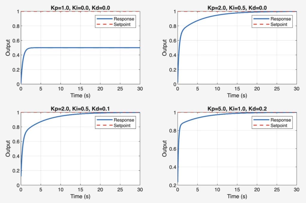
PID Loop in Code — Matlab Example
Here’s a clean, reusable discrete-time PID loop implementation in Matlab:
clc
clear
close all

dt = 0.01;
t = 0:dt:30;
setpoint = 1;

params = [
    1.0 0.0 0.0
    2.0 0.5 0.0
    2.0 0.5 0.1
    5.0 1.0 0.2
];

tau = 1.0;

figure

for k = 1:size(params,1)

    Kp = params(k,1);
    Ki = params(k,2);
    Kd = params(k,3);

    y = 0;
    integral = 0;
    prev_error = 0;

    y_log = zeros(length(t),1);

    for i = 1:length(t)
        error = setpoint - y;

        P = Kp * error;
        integral = integral + error * dt;
        I = Ki * integral;
        D = Kd * (error - prev_error) / dt;

        u = P + I + D;

        dy = (-y + u) / tau;
        y = y + dy * dt;

        prev_error = error;
        y_log(i) = y;
    end

    subplot(2,2,k)
    ylim([0 2])
    plot(t, y_log, 'LineWidth', 2)
    hold on
    plot(t, setpoint*ones(size(t)), '--r', 'LineWidth', 1.5)
    grid on
    title(sprintf('Kp=%.1f, Ki=%.1f, Kd=%.1f', Kp, Ki, Kd))
    xlabel('Time (s)')
    ylabel('Output')
    legend('Response','Setpoint')
end
💡 Key improvements over a basic PID:
- Derivative on measurement (not error) → prevents derivative kick on setpoint changes
- Anti-windup via back-calculation → prevents integral windup when output saturates
- Output clamping → keeps the control signal within actuator limits
Limitations of the PID Loop
For all its power, the PID loop has real constraints that engineers must understand:
| Limitation | Why It Matters |
|---|---|
| Linear assumption | PID is designed for linear systems; performance degrades with strong nonlinearities |
| SISO only | Standard PID handles one variable at a time; multi-variable systems need multiple loops or advanced methods (e.g., MPC) |
| Dead time sensitivity | Large process delays make PID tuning difficult and can cause instability |
| Noise sensitivity | Derivative term requires filtering, which introduces lag |
| Reactive, not proactive | PID only responds to errors after they occur — it has no feedforward capability without modification |
| Manual tuning burden | Optimal gains often require experience, iteration, or system modeling |
When the PID loop isn’t enough, engineers turn to cascade PID, feedforward + PID, Model Predictive Control (MPC), adaptive control, or fuzzy logic control.
FAQ — PID Loop Explained
Q1. What does PID loop stand for?
PID stands for Proportional, Integral, Derivative. The “loop” refers to the closed feedback loop in which the controller continuously measures the output, compares it to the setpoint, and adjusts its output to minimize the error.
Q2. What is the difference between a PID loop and a PID controller?
The terms are often used interchangeably. Technically, the PID controller is the algorithm or device, while the PID loop refers to the complete closed-loop system — including the controller, plant, sensors, and feedback path working together.
Q3. Why does a PID loop oscillate?
Oscillation in a PID loop is almost always caused by too high a proportional gain (Kp). The controller overcorrects in one direction, which causes an overshoot, then overcorrects back, creating a continuous back-and-forth cycle. The fix is to reduce Kp and optionally increase Kd for damping.
Q4. What is integral windup in a PID loop?
Integral windup occurs when the PID loop’s integral term accumulates an excessively large value during a period when the actuator is saturated (maxed out). When the system eventually approaches the setpoint, the wound-up integral causes severe overshoot. Anti-windup techniques — such as clamping the integral or back-calculation — prevent this.
Q5. How do I tune a PID loop without a model?
The most practical model-free method is the Ziegler-Nichols closed-loop method: increase Kp until the system oscillates at constant amplitude, record the ultimate gain (Ku) and ultimate period (Tu), then use the Ziegler-Nichols table to calculate starting values for Kp, Ki, and Kd. Fine-tune from there with manual adjustment.
Q6. When should I use PI instead of PID?
Use a PI loop when the process signal is noisy (making derivative action unreliable), when the system is relatively slow-responding (so derivative action adds little benefit), or when simplicity is preferred. PI is the most commonly used configuration in industrial process control for exactly these reasons.
Q7. Can a PID loop control nonlinear systems?
A PID loop can work on mildly nonlinear systems if tuned conservatively. For strongly nonlinear systems, gain scheduling (different PID parameters at different operating points), adaptive PID, or advanced methods like Model Predictive Control (MPC) are more appropriate.
References and Further Reading
This article is part of the Mechatronics Engineering fundamentals series. If you found this PID loop explained guide helpful, feel free to share it or leave a question in the comments below.