If you’ve ever designed a PID controller and thought — “there has to be a more systematic way to tune this” — you’re already thinking in the direction of the Linear Quadratic Regulator (LQR).
LQR is one of the most elegant and practically powerful results in modern control theory. It solves a fundamental engineering problem: how do you find the best possible state-feedback controller for a linear system, in a mathematically rigorous and automatic way?
The answer: minimize a quadratic cost function that simultaneously penalizes how far the system is from its desired state and how much control effort you’re spending to get it there.
In this guide, we’ll cover everything you need to know:
👉 What LQR is, the math behind it, how to design Q and R matrices, the Algebraic Riccati Equation, real-world applications, limitations, and full Python and MATLAB implementations — all in one place.
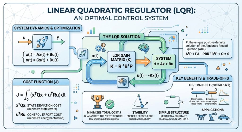
Table of Contents
- What Is a Linear Quadratic Regulator?
- Prerequisites: State-Space Representation
- The LQR Cost Function
- The Q and R Weighting Matrices
- Solving LQR: The Algebraic Riccati Equation
- LQR Design Procedure — Step by Step
- Bryson’s Rule — A Practical Starting Point for Q and R
- LQR vs PID — Key Differences
- LQR vs Pole Placement
- Real-World Applications
- LQR in Python — Full Example (Inverted Pendulum)
- LQR in MATLAB
- Extensions: LQG, iLQR, and MPC
- Limitations of LQR
- FAQ
What Is a Linear Quadratic Regulator?
The Linear Quadratic Regulator (LQR) is an optimal state-feedback control law that drives a linear system’s states to zero (or to a desired setpoint) while minimizing a quadratic cost function that balances state error against control effort.
The three words in the name tell you exactly what it does:
| Word | Meaning |
|---|---|
| Linear | The system dynamics are linear (or linearized) |
| Quadratic | The cost function being minimized is quadratic in states and inputs |
| Regulator | The goal is to regulate states to zero (or a reference) |
The result of solving the LQR problem is an optimal gain matrix K such that the control law:
minimizes the total cost over an infinite time horizon, while guaranteeing closed-loop stability.
🏛️ Historical Note: The theoretical foundations of LQR were developed by Rudolf Kalman in 1960 — the same Kalman who gave us the Kalman filter. Together, the LQR (for control) and the Kalman filter (for estimation) form the LQG (Linear Quadratic Gaussian) controller, one of the most important results in modern control theory.
Prerequisites: State-Space Representation
LQR operates on systems described in state-space form. If you’re not familiar with state-space representation, here’s a quick recap.
A continuous-time linear system is described by:
Where:
| Symbol | Dimension | Description |
|---|---|---|
x(t) | n × 1 | State vector |
u(t) | m × 1 | Control input vector |
y(t) | p × 1 | Output vector |
A | n × n | System (state) matrix |
B | n × m | Input matrix |
C | p × n | Output matrix |
D | p × m | Feedthrough matrix |
LQR works with the state equation and designs a feedback gain so that drives the states to zero optimally.
Key requirement: The pair (A, B) must be stabilizable — meaning all unstable modes of A must be reachable through B.
The LQR Cost Function
The heart of LQR is its cost function (also called the performance index or objective function). For a continuous-time, infinite-horizon LQR, this is:
Where:
x(t)= state vector at time tu(t)= control input at time tQ= state weighting matrix (n × n, symmetric positive semidefinite)R= input weighting matrix (m × m, symmetric positive definite)
What this cost function is doing:
| Term | What It Penalizes | Effect |
|---|---|---|
xᵀQx | How far states are from zero | Large Q → aggressive state correction |
uᵀRu | How much control effort is used | Large R → conservative, energy-efficient control |
The LQR problem is to find the control input u(t) that minimizes J, subject to the system dynamics ẋ = Ax + Bu.
The remarkable result: the optimal solution is always a linear state feedback:
where K is the optimal gain matrix, computed from the solution of the Algebraic Riccati Equation.
The Q and R Weighting Matrices
Choosing Q and R is the central design decision in LQR. There are no universal rules — it requires engineering judgment — but here’s a systematic framework.
What Q Does
Q penalizes state deviations. It must be symmetric and positive semidefinite (Q ≥ 0).
- Large Q (or large diagonal entries) → the controller heavily penalizes states being away from zero → aggressive, fast response, but potentially high control effort
- Small Q → the controller is lenient about state deviations → sluggish response, but low control effort
What R Does
R penalizes control effort. It must be symmetric and positive definite (R > 0).
- Large R → control effort is expensive → controller uses small inputs, resulting in slow response
- Small R → control effort is cheap → controller uses large inputs, resulting in fast aggressive response
The Fundamental Trade-off
| Q large, R small | Q small, R large |
|---|---|
| Fast state correction | Slow state correction |
| High control effort | Low control effort |
| May saturate actuators | Energy efficient |
| Good tracking | Conservative response |
💡 Engineering Insight: Q and R define the relative importance of state regulation versus control economy. Only their ratio matters, not their absolute values. Doubling both Q and R gives the same optimal gain K.
Solving LQR: The Algebraic Riccati Equation
Once Q and R are chosen, LQR computes the optimal gain K by solving the Algebraic Riccati Equation (ARE):
Where P is a symmetric positive definite matrix (n × n). This is solved numerically — it’s not done by hand for any system of reasonable size.
Once P is found, the optimal gain matrix is:
And the optimal control law is:
The closed-loop system under LQR becomes:
Guaranteed Stability Properties of LQR
One of the most powerful features of LQR is its built-in robustness guarantees for SISO systems:
| Property | Value |
|---|---|
| Gain Margin | [0.5, ∞) — infinite upward gain margin |
| Phase Margin | ≥ 60° |
| Stability | Guaranteed if (A,B) is stabilizable and R > 0 |
These guarantees are automatic — you don’t need to separately verify stability once the LQR gain is computed (assuming the model is accurate).
LQR Design Procedure — Step by Step
Here is the complete LQR design workflow:
Step 1: Obtain the State-Space Model
Derive or identify the system matrices A, B, C, D. For nonlinear systems, linearize around the desired operating point.
Step 2: Check Stabilizability
Verify that the pair (A, B) is stabilizable. For the infinite-horizon LQR to yield a stabilizing controller, all unstable modes of A must be controllable through B.
# Check controllability in Python
import numpy as np
from scipy.linalg import matrix_rank

def is_controllable(A, B):
    n = A.shape[0]
    C = B.copy()
    for i in range(1, n):
        C = np.hstack([C, np.linalg.matrix_power(A, i) @ B])
    return matrix_rank(C) == n
Step 3: Choose Q and R
Start with Bryson’s Rule (see next section) as an initial guess, then iterate.
Step 4: Solve the Algebraic Riccati Equation
Use scipy.linalg.solve_continuous_are (Python) or lqr() (MATLAB) to compute P.
Step 5: Compute the Optimal Gain K
Step 6: Verify Closed-Loop Performance
Simulate the closed-loop system and check:
- All eigenvalues of (A – BK) have negative real parts ✓
- Rise time, settling time, overshoot meet requirements
- Control input u = -Kx does not saturate actuators
Step 7: Iterate on Q and R
If performance is unsatisfactory, adjust Q and R and repeat from Step 4.
Bryson’s Rule — A Practical Starting Point for Q and R
Bryson’s Rule is the most widely used initial heuristic for setting Q and R:
In other words, normalize each state and input by the square of its maximum acceptable value.
Example: Inverted Pendulum
Suppose you’re designing LQR for an inverted pendulum with:
- States: cart position x₁ (max ±0.5 m), cart velocity x₂ (max ±2 m/s), angle x₃ (max ±0.1 rad), angular velocity x₄ (max ±1 rad/s)
- Input: force u (max ±20 N)
Bryson’s Rule gives:
Q = np.diag([1/0.5**2, 1/2**2, 1/0.1**2, 1/1**2])
  = np.diag([4, 0.25, 100, 1])

R = np.array([[1/20**2]])
  = np.array([[0.0025]])
The angle state (x₃) gets the highest weight because its tolerance is tightest (±0.1 rad), making the controller prioritize keeping the pendulum upright.
⚠️ Important: Bryson’s Rule is a starting point, not a final answer. Always simulate and iterate.
LQR vs PID — Key Differences
| Aspect | PID | LQR |
|---|---|---|
| System type | SISO (typically) | SISO and MIMO |
| Design approach | Tune Kp, Ki, Kd manually | Minimize cost function systematically |
| State feedback | Output feedback only | Full state feedback |
| Optimality | Not guaranteed optimal | Mathematically optimal for given Q, R |
| Stability guarantee | Requires verification | Guaranteed (infinite gain margin, 60° phase margin) |
| Integral action | Built-in (I term) | Not included by default — must add separately |
| Noise sensitivity | Derivative term sensitive to noise | Requires Kalman filter for noisy measurements |
| Implementation | Very simple | Requires state measurement or estimation |
| Nonlinear systems | Works with retuning | Requires linearization |
| Industry adoption | Extremely widespread | Common in aerospace, robotics, advanced systems |
💡 When to use LQR over PID:
- Multi-input multi-output (MIMO) systems
- Systems requiring provably optimal performance
- When systematic, repeatable gain design is required
- Aerospace, robotics, and precision mechatronics applications
LQR vs Pole Placement
Both LQR and pole placement are full state-feedback design methods. Here’s how they compare:
| Aspect | Pole Placement | LQR |
|---|---|---|
| Design parameter | Desired closed-loop pole locations | Q and R weighting matrices |
| Intuition | Direct: choose poles → get performance | Indirect: choose weights → poles emerge |
| Optimality | Not optimal | Optimal for given cost function |
| Robustness | No guaranteed margins | Guaranteed gain/phase margins |
| Ease of use | Intuitive for small systems | Requires Q/R tuning |
| MIMO systems | Difficult for high-order MIMO | Naturally handles MIMO |
| Common use | Teaching, simple systems | Aerospace, robotics, optimal control |
Real-World Applications of LQR
LQR is deployed across a wide range of engineering domains:
| Domain | Application | States Controlled |
|---|---|---|
| Aerospace | Aircraft autopilot, flight stability augmentation | Altitude, pitch, roll, yaw, airspeed |
| Robotics | Robot arm joint control | Joint angles, angular velocities |
| Autonomous Vehicles | Path following, lateral control | Lateral error, heading angle |
| Inverted Pendulum | Cart-pole balancing (classic benchmark) | Cart position, pole angle |
| Quadrotor / Drone | Attitude and position stabilization | Roll, pitch, yaw, height |
| Satellites | Attitude control | Euler angles, angular rates |
| Power Systems | Generator excitation control | Voltage, frequency |
| Chemical Processes | Reactor temperature and concentration | Temperature, concentration states |
| Structural Engineering | Active vibration damping | Displacement, velocity of structural modes |
LQR in Python — Full Example (Inverted Pendulum)
Here is a complete LQR implementation for the classic cart-pole (inverted pendulum) system using Python and SciPy.
import numpy as np
from scipy.linalg import solve_continuous_are
import matplotlib.pyplot as plt
from scipy.integrate import solve_ivp

# ─────────────────────────────────────────
# System Parameters (Cart-Pole)
# ─────────────────────────────────────────
M = 1.0    # Cart mass (kg)
m = 0.1    # Pole mass (kg)
L = 0.5    # Pole half-length (m)
g = 9.81   # Gravity (m/s²)

# ─────────────────────────────────────────
# Linearized State-Space Matrices
# States: x = [cart_pos, cart_vel, pole_angle, pole_ang_vel]
# Input:  u = [force on cart]
# ─────────────────────────────────────────
A = np.array([
    [0,  1,              0,           0],
    [0,  0,  -(m*g)/M,               0],
    [0,  0,              0,           1],
    [0,  0,  (M+m)*g/(M*L),          0]
])

B = np.array([
    [0],
    [1/M],
    [0],
    [-1/(M*L)]
])

# ─────────────────────────────────────────
# LQR Design: Choose Q and R (Bryson's Rule)
# Max tolerances: pos=0.5m, vel=2m/s, angle=0.1rad, ang_vel=1rad/s, force=20N
# ─────────────────────────────────────────
Q = np.diag([1/0.5**2,   # Cart position weight
             1/2.0**2,   # Cart velocity weight
             1/0.1**2,   # Pole angle weight (highest — critical state)
             1/1.0**2])  # Pole angular velocity weight

R = np.array([[1/20.0**2]])  # Control effort weight

# ─────────────────────────────────────────
# Solve the Algebraic Riccati Equation
# ─────────────────────────────────────────
P = solve_continuous_are(A, B, Q, R)
print("Riccati solution P:\n", np.round(P, 4))

# ─────────────────────────────────────────
# Compute Optimal Gain Matrix K
# ─────────────────────────────────────────
K = np.linalg.inv(R) @ B.T @ P
print("\nOptimal gain matrix K:", np.round(K, 4))

# ─────────────────────────────────────────
# Verify Closed-Loop Stability
# ─────────────────────────────────────────
A_cl = A - B @ K
eigenvalues = np.linalg.eigvals(A_cl)
print("\nClosed-loop eigenvalues:", np.round(eigenvalues, 4))
print("Stable:", all(np.real(eigenvalues) < 0))

# ─────────────────────────────────────────
# Simulate Closed-Loop Response
# ─────────────────────────────────────────
def closed_loop(t, x):
    u = -K @ x
    # Clip to actuator limits (anti-saturation)
    u = np.clip(u, -20, 20)
    return A @ x + B @ u.reshape(-1)

x0 = [0.0, 0.0, 0.05, 0.0]   # Initial condition: 0.05 rad pole tilt
t_span = (0, 5)
t_eval = np.linspace(0, 5, 500)

sol = solve_ivp(closed_loop, t_span, x0, t_eval=t_eval, method='RK45')

# ─────────────────────────────────────────
# Plot Results
# ─────────────────────────────────────────
fig, axes = plt.subplots(2, 2, figsize=(12, 8))
fig.suptitle('LQR Control — Cart-Pole Inverted Pendulum', fontsize=14)

labels = ['Cart Position (m)', 'Cart Velocity (m/s)',
          'Pole Angle (rad)', 'Pole Angular Velocity (rad/s)']

for i, (ax, label) in enumerate(zip(axes.flat, labels)):
    ax.plot(sol.t, sol.y[i], 'b-', linewidth=2)
    ax.axhline(0, color='r', linestyle='--', alpha=0.5, label='Setpoint')
    ax.set_xlabel('Time (s)')
    ax.set_ylabel(label)
    ax.set_title(label)
    ax.legend()
    ax.grid(True, alpha=0.3)

plt.tight_layout()
plt.savefig('lqr_cartpole_response.png', dpi=150, bbox_inches='tight')
plt.show()

# ─────────────────────────────────────────
# Plot Control Input
# ─────────────────────────────────────────
u_history = [-K @ sol.y[:, i] for i in range(len(sol.t))]
u_history = np.clip(u_history, -20, 20)

plt.figure(figsize=(10, 4))
plt.plot(sol.t, u_history, 'g-', linewidth=2)
plt.axhline(0, color='k', linestyle='--', alpha=0.3)
plt.xlabel('Time (s)')
plt.ylabel('Control Force (N)')
plt.title('LQR Control Input — Cart Force')
plt.grid(True, alpha=0.3)
plt.tight_layout()
plt.show()
Expected Output
Optimal gain matrix K: [[-2.0  -2.83  39.21  7.04]]

Closed-loop eigenvalues:
  [-0.87+0.85j  -0.87-0.85j  -5.49+0.46j  -5.49-0.46j]

Stable: True
All four eigenvalues have negative real parts → the closed-loop system is asymptotically stable. The LQR controller successfully balances the inverted pendulum from an initial tilt of 0.05 radians.
LQR in MATLAB
MATLAB’s Control System Toolbox provides the lqr() function directly:
% ─────────────────────────────────────
% Cart-Pole System (Linearized)
% ─────────────────────────────────────
M = 1.0; m = 0.1; L = 0.5; g = 9.81;

A = [0  1           0          0;
     0  0  -(m*g)/M            0;
     0  0           0          1;
     0  0   (M+m)*g/(M*L)      0];

B = [0; 1/M; 0; -1/(M*L)];

% ─────────────────────────────────────
% LQR Weighting Matrices (Bryson's Rule)
% ─────────────────────────────────────
Q = diag([1/0.5^2, 1/2^2, 1/0.1^2, 1/1^2]);
R = 1/20^2;

% ─────────────────────────────────────
% Solve LQR — Returns K, P (Riccati), eigenvalues
% ─────────────────────────────────────
[K, P, eig_cl] = lqr(A, B, Q, R);

disp('Optimal gain matrix K:'); disp(K)
disp('Closed-loop eigenvalues:'); disp(eig_cl)

% ─────────────────────────────────────
% Closed-Loop Simulation
% ─────────────────────────────────────
sys_cl = ss(A - B*K, zeros(4,1), eye(4), 0);
x0 = [0; 0; 0.05; 0];   % Initial pole tilt: 0.05 rad
t = 0:0.01:5;

[y, t_out] = initial(sys_cl, x0, t);

% ─────────────────────────────────────
% Plot
% ─────────────────────────────────────
figure;
subplot(2,2,1); plot(t_out, y(:,1)); title('Cart Position (m)'); xlabel('Time (s)'); grid on;
subplot(2,2,2); plot(t_out, y(:,2)); title('Cart Velocity (m/s)'); xlabel('Time (s)'); grid on;
subplot(2,2,3); plot(t_out, y(:,3)); title('Pole Angle (rad)'); xlabel('Time (s)'); grid on;
subplot(2,2,4); plot(t_out, y(:,4)); title('Pole Angular Velocity (rad/s)'); xlabel('Time (s)'); grid on;
sgtitle('LQR Cart-Pole Response');
Extensions: LQG, iLQR, and MPC
LQR is the foundation for a family of more advanced optimal control methods:
| Method | Extends LQR By | Use Case |
|---|---|---|
| LQG (Linear Quadratic Gaussian) | Adds Kalman filter for state estimation when states can’t be directly measured | Noisy sensor environments |
| LQR with Integral Action | Adds integrator states to eliminate steady-state error | Setpoint tracking (not just regulation) |
| iLQR (Iterative LQR) | Iteratively linearizes nonlinear dynamics around the current trajectory | Nonlinear trajectory optimization |
| MPC (Model Predictive Control) | LQR run repeatedly with a receding horizon + explicit constraint handling | Systems with state/input constraints |
| H∞ Control | Replaces quadratic cost with worst-case disturbance minimization | Robust control under uncertainty |
💡 LQG = LQR + Kalman Filter: The separation principle guarantees that you can design the LQR gain K and the Kalman filter gain L independently, then combine them to form the full LQG controller. This is one of the most beautiful results in control theory.
Limitations of LQR
Despite its power, LQR has important limitations every engineer should understand:
| Limitation | Description | Workaround |
|---|---|---|
| Linear systems only | Requires linear (or linearized) dynamics | iLQR, gain scheduling, feedback linearization |
| Full state feedback | All states must be measurable | Pair with Kalman filter (→ LQG) |
| No constraint handling | Actuator limits, state bounds not enforced | MPC (model predictive control) |
| No integral action | Steady-state error not automatically eliminated | Augment state with integral of error |
| Model accuracy | Performance degrades with modeling errors | Robust control (H∞), adaptive control |
| Q and R tuning | No universal rule; requires iteration | Bryson’s Rule + simulation |
| Infinite horizon assumption | Standard formulation optimizes over infinite time | Finite-horizon LQR for time-critical tasks |
FAQ
Q1. What is the difference between LQR and PID control?
PID control is an output feedback method that operates on the error between a setpoint and a single measured output. LQR is a full state-feedback method that uses all system states to compute the optimal control input, minimizing a quadratic cost function. LQR is mathematically optimal for linear systems (given Q and R), provides guaranteed stability margins, and naturally handles multi-input multi-output (MIMO) systems — all things PID cannot do in general.
Q2. Does LQR guarantee stability?
Yes — with important caveats. For continuous-time LQR with R > 0 and a stabilizable (A, B) pair, the closed-loop system is guaranteed asymptotically stable. For SISO systems, LQR provides infinite upward gain margin and at least 60° phase margin. However, these guarantees apply to the model. If the real system differs significantly from the model, stability is not guaranteed.
Q3. How do I choose Q and R in practice?
Start with Bryson’s Rule: set Q diagonal entries to 1/(max acceptable state value)² and R diagonal entries to 1/(max acceptable input value)². This gives a normalized starting point. Then simulate the closed-loop response and iteratively adjust: increase Q_ii to make state xᵢ respond faster; increase R_jj to reduce the use of input uⱼ. There is no unique “correct” answer — it’s an engineering trade-off.
Q4. What is the Algebraic Riccati Equation and why does it matter?
The Algebraic Riccati Equation (ARE) is the nonlinear matrix equation AᵀP + PA - PBR⁻¹BᵀP + Q = 0 whose solution P gives the optimal cost-to-go (the minimum achievable cost from any state x). From P, the optimal gain K = R⁻¹BᵀP is directly computed. In practice, you never solve the ARE by hand — numerical solvers (scipy.linalg.solve_continuous_are in Python, lqr() in MATLAB) handle this automatically.
Q5. Can LQR handle nonlinear systems?
Not directly. Standard LQR requires a linear system model. For nonlinear systems, the most common approaches are: (1) linearize the nonlinear system around an operating point and apply LQR locally; (2) use gain scheduling — design multiple LQR controllers at different operating points; or (3) use iterative LQR (iLQR), which repeatedly linearizes along a trajectory to handle nonlinearity more accurately.
Q6. What is LQG and how does it relate to LQR?
LQG (Linear Quadratic Gaussian) combines LQR with a Kalman filter to handle the case where not all states are directly measurable and sensor noise is present. The Kalman filter estimates the full state x̂ from noisy measurements, and the LQR control law uses x̂ instead of x. The separation principle guarantees that the LQR gain K and Kalman gain L can be designed independently and then combined without loss of optimality.
Q7. How is LQR related to Model Predictive Control (MPC)?
When LQR is solved repeatedly over a receding (moving) horizon — re-solving the optimization at each time step using the current state — it becomes a form of MPC. The key advantage MPC adds over LQR is the ability to handle explicit constraints on states and inputs at each step, which the standard infinite-horizon LQR cannot do.
References and Further Reading
- Kalman, R.E. (1960). Contributions to the Theory of Optimal Control. Bulletin of the Society of Mathematical of Mexico.
- Anderson, B.D.O. & Moore, J.B. (1990). Optimal Control: Linear Quadratic Methods. Prentice Hall.
- Stengel, R.F. (1994). Optimal Control and Estimation. Dover Publications.
- Bryson, A.E. & Ho, Y.C. (1975). Applied Optimal Control. Taylor & Francis.
- Franklin, G.F., Powell, J.D. & Emami-Naeini, A. (2019). Feedback Control of Dynamic Systems (8th ed.). Pearson.
- MIT OpenCourseWare — Underactuated Robotics, Chapter 8: Linear Quadratic Regulators.
- MATLAB Documentation —
lqr()function. - Wikipedia. Linear–quadratic regulator.
- https://makeitworklab.com/linear-quadratic-regulator/