When starting with Mechatronics systems, it is tempting to jump directly into motors, sensors, and complex control algorithms. However, every serious engineering journey begins with a simple and fundamental experiment.

In the Arduino ecosystem, that experiment is turning on the built-in LED.

Although this may look trivial, this small task introduces essential concepts: digital output control, pin configuration, timing, and program structure. More importantly, it establishes the foundation for understanding how software interacts with physical hardware — the core principle of control engineering.

Why Start with the Built-in LED?

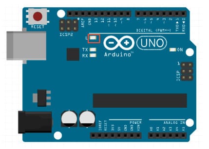
Most Arduino boards, including the Arduino Uno, contain an onboard LED connected internally to a digital pin. On the Arduino Uno, this LED is connected to digital pin 13.

Using the built-in LED has several advantages:

• No external wiring is required
• No resistor calculation is needed
• No risk of incorrect circuit connections
• Immediate hardware feedback

From a systems perspective, the LED represents a simple actuator. When we command HIGH or LOW from software, we are directly manipulating a physical output state.

This is the most basic example of:

Input (program instruction) → Processing → Physical Output

That relationship is the backbone of all embedded and control systems.

System Principles

Before writing code, it is important to understand what we are actually doing.

An LED is a diode that emits light when current flows through it. In digital control terms:

• HIGH → 5V output → LED ON
• LOW → 0V output → LED OFF

In embedded systems, a digital output pin behaves like a switch controlled by software. When configured as OUTPUT, the microcontroller can source or sink current through that pin.

This experiment is essentially commanding the microcontroller to behave as a digitally controlled switch.

Hardware and Software Requirement

• Arduino Uno
• USB cable
• Arduino IDE
• Matlab (optional)

Schematic Diagram

• It’s so simple. Connect Arduino Uno to your laptop using USB cable

Arduino code

Put the below code in your Arduino IDE and see the result.

Then you will see built-in LED blinking in line with the code.

const int ledPin = LED_BUILTIN;

void setup() {
  pinMode(ledPin, OUTPUT);
}

void loop() {
  digitalWrite(ledPin, HIGH);   // Turn LED ON
  delay(1000);                  // Wait 1000 ms
  digitalWrite(ledPin, LOW);    // Turn LED OFF
  delay(1000);                  // Wait 1000 ms
}

Engineering analysis

Signal output

This is not random blinking. You just generated a square wave signal.

Let’s analyze it as engineers.

Total period

Frequency :

The duty cycle describes how long the signal stays HIGH during one period.

Without realizing it, you just built a low-frequency digital signal generator.

If you have access to an oscilloscope, you can directly observe the waveform by probing pin 13. However, many beginners may not own an oscilloscope, as it can be relatively expensive.

For that reason, I’ve included the ideal digital signal graph below.

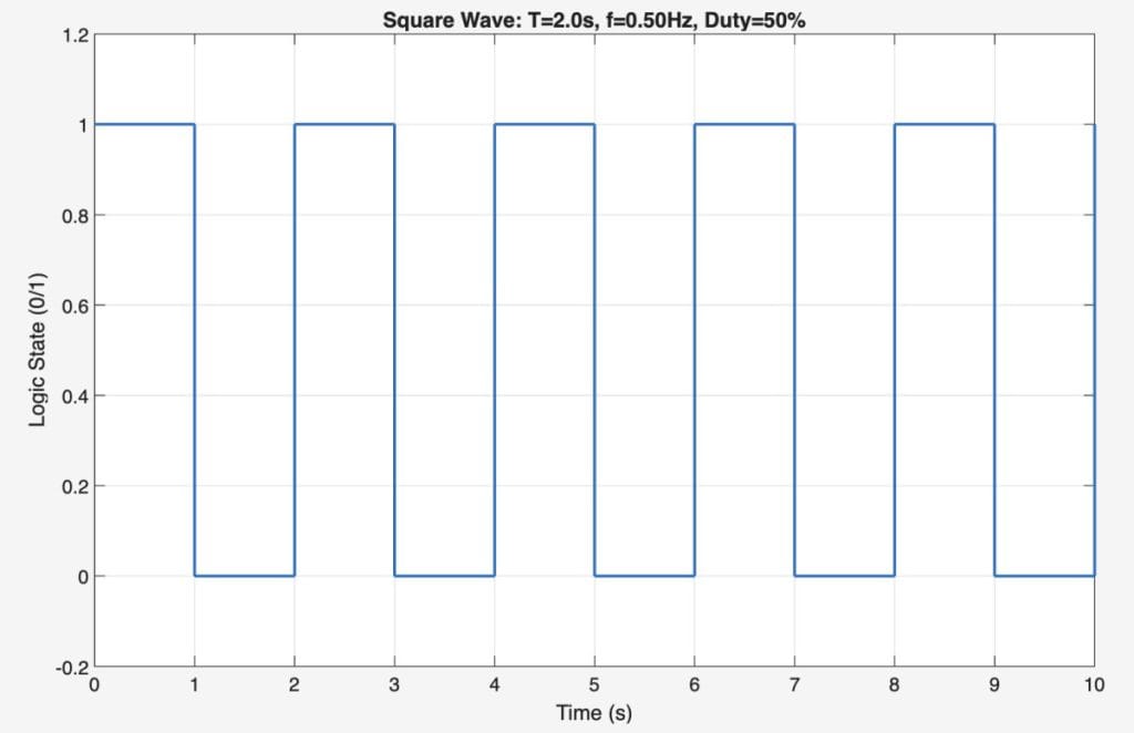
Keep in mind that this graph represents an ideal square wave. In real hardware, the waveform will not be perfectly sharp or clean. Noise, signal delay, switching transients, and other disturbances can slightly distort the edges and timing of the signal.

In practical systems, digital signals are influenced by:

• Electrical noise
• Switching delays
• Finite rise and fall times
• Hardware limitations

Therefore, what you see in simulation or theoretical plots may differ slightly from measurements taken in real circuits.

You can easily reproduce this ideal waveform in MATLAB using the code shown below.

clc; clear; close all;

% ===== Square wave condition =====
T = 2;              % period [s]
f = 1/T;            % frequency [Hz] = 0.5 Hz
duty = 50;          % duty cycle [%]
A = 1;              % logic amplitude (0/1)
Ncycles = 5;        % Number of cycles

% ===== sampling setting =====
Fs = 200;           % sampling frequency [Hz] 
t_end = Ncycles*T;  % Total time
t = 0:1/Fs:t_end;   % time vector

% ===== Square wave signal generation =====
% square()
x = (square(2*pi*f*t, duty) + 1)/2;   % 0 or 1

% ===== floating =====
figure;
stairs(t, x, "LineWidth", 1.5);
grid on;
ylim([-0.2 1.2]);
xlabel("Time (s)");
ylabel("Logic State (0/1)");
title(sprintf("Square Wave: T=%.1fs, f=%.2fHz, Duty=%d%%", T, f, duty));

% ===== output logging =====
Ton  = (duty/100)*T;
Toff = T - Ton;
fprintf("Period T = %.3f s\n", T);
fprintf("Frequency f = %.3f Hz\n", f);
fprintf("Ton = %.3f s, Toff = %.3f s (Duty = %d%%)\n", Ton, Toff, duty);

Changing Frequency

Let’s examine how the LED behavior changes when we vary the frequency. The blinking pattern is not fixed — it can be easily adjusted by modifying the delay values in the code.

In this experiment, the frequency was set to:

• 0.5 Hz
• 1 Hz
• 5 Hz

As the frequency increases, the LED toggles more rapidly, reducing the visible blinking interval.

Watch the video below to observe how the LED behavior changes at each frequency setting.

const int ledPin = LED_BUILTIN;

void setup() {
  pinMode(ledPin, OUTPUT);
}

void loop() {
  digitalWrite(ledPin, HIGH);   // Turn LED ON
  delay(1000);                  // Wait 1000 ms , change if you want to modify frequency
  digitalWrite(ledPin, LOW);    // Turn LED OFF
  delay(1000);                  // Wait 1000 ms, change if you want to modify frequency
}

Changing Duty cycle

You can also experiment by changing the duty cycle. As discussed earlier, the duty cycle represents the percentage of time the signal remains HIGH during one complete period.

Unlike frequency, which determines how fast the signal repeats, the duty cycle determines how long the LED stays ON within each cycle.

In this experiment, the duty cycle was adjusted to:

• 50%
• 25%
• 10%

When the duty cycle decreases, the ON time becomes shorter while the total period remains constant (if frequency is unchanged). As a result, the LED appears to stay ON for a smaller portion of each cycle.

Watch the video below to observe how the LED behavior changes as the duty cycle varies.