In the world of high-performance robotics and aerospace, one name stands above the rest: Maxon Motor. Known for their ironless winding and extreme power density, Maxon motors (like those used on the Mars Rovers) require precise control to truly shine.
Today, we will break down the journey from raw physics to a fully tuned PID Control system using the Maxon DCX 22 L (12V) as our reference model.
1. Defining the Plant: The Maxon DCX 22 L
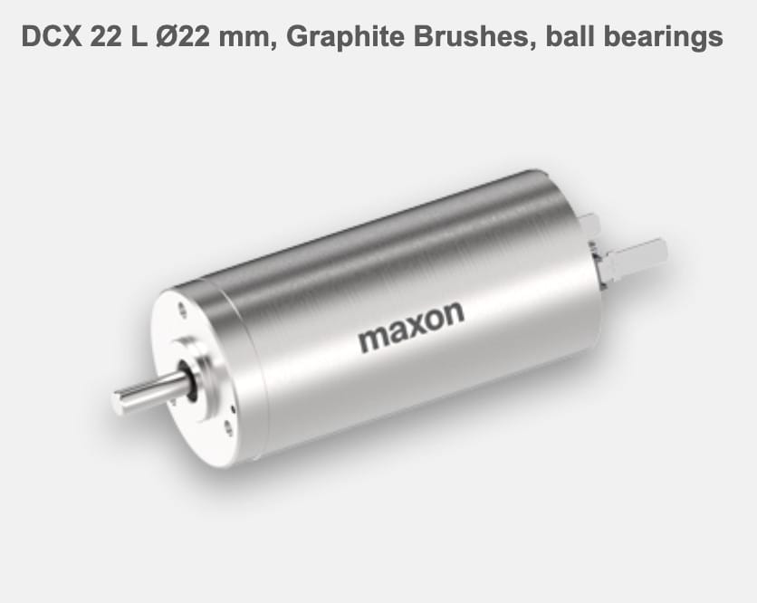
Before writing a single line of code, we must understand the “Plant”—the physical motor. The DCX 22 L is a high-performance graphite-brushed motor. Based on its datasheet, here are the parameters we’ll use for our mathematical model:
| Parameter | Symbol | Value | Unit |
| Nominal Voltage | 48 | V | |
| Terminal Resistance | 7.39 | ||
| Terminal Inductance | 0.746 | mH | |
| Torque Constant | 45.2 | mNm/A | |
| Speed Constant | 211 | rpm/V | |
| Rotor Inertia | 8.85 | gcm² |
2. The Mathematical Model (Physics Equations)
The behavior of a DC motor is governed by two coupled differential equations: the electrical and the mechanical.
The Electrical Loop (KVL)
The input voltage must overcome the resistance, the inductance, and the Back-EMF generated by the rotation:
The Mechanical Loop (Newton’s 2nd Law)
The torque produced accelerates the rotor’s inertia while overcoming viscous friction :
By applying the Laplace Transform, we derive the Transfer Function , representing the ratio of Output Speed to Input Voltage :
3. Implementing PID Control
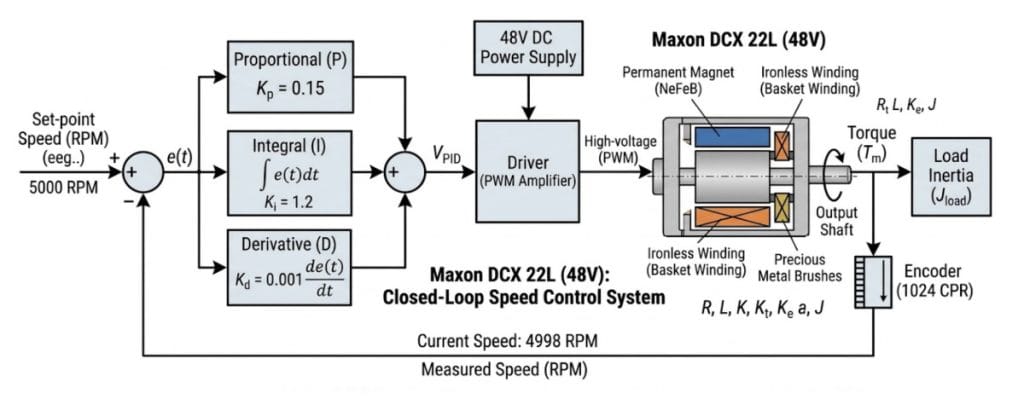
To reach a target speed of 3,000 RPM accurately under varying loads, we implement a PID (Proportional-Integral-Derivative) controller:
- P (Proportional): Reacts to the current error. High decreases rise time.
- I (Integral): Eliminates steady-state error. Ensures the motor hits exactly 3,000 RPM.
- D (Derivative): Predicts future error. Dampens oscillations and prevents overshoot.
below picture explain how DC motor PID feedback loop looks like (generated by AI)
4. MATLAB Simulation Script
The following MATLAB code simulates the closed-loop response of the Maxon DCX 22 L.
%% Maxon DCX 22 L PID Speed Control Simulation
clear all; close all; clc;

% --- Motor Parameters ---
R = 2.32;             % [Ohm]
L = 0.22e-3;          % [H]
Kt = 23.4e-3;         % [Nm/A]
Ke = 23.4e-3;         % [V/(rad/s)]
J = 4.21e-7;          % [kg*m^2]
b = 1.0e-6;           % Estimated Friction

% --- Transfer Function ---
s = tf('s');
Motor_TF = Kt / ((L*s + R)*(J*s + b) + Kt*Ke);

% --- PID Controller Tuning ---
Kp = 0.08;
Ki = 0.6;
Kd = 0.0005;
C = pid(Kp, Ki, Kd);

% --- Closed-Loop System ---
sys_cl = feedback(C * Motor_TF, 1);

% --- Simulation (Target: 3000 RPM) ---
target_rpm = 3000;
target_rad_s = target_rpm * (2 * pi / 60);
t = 0:0.0001:0.1;

[y, t] = step(target_rad_s * sys_cl, t);
actual_rpm = y * (60 / (2 * pi));

% --- Plotting Results ---
figure('Color', 'w');
plot(t, actual_rpm, 'LineWidth', 2);
hold on;
yline(target_rpm, 'r--', 'Target 3000 RPM');
grid on;
title('Maxon DCX 22 L Speed Response via PID');
xlabel('Time (s)'); ylabel('Speed (RPM)');
legend('Actual Response', 'Setpoint');
5. From Rotation to Translation: Controlling a Linear Actuator
In many industrial applications, a DC motor doesn’t just spin; it drives a Ball Screw to convert rotary motion into linear displacement.
The Challenge: Suppose we need to move a carriage 1 meter in exactly 5 seconds using our Maxon DCX 22L (48V) and a ball screw with a 5mm lead. This requires shifting from simple speed control to High-Precision Position Control.

The 4-Step Professional PID Tuning Procedure
To achieve this “1 meter in 5 seconds” goal without damaging the mechanical stops or vibrating the load, we follow a systematic tuning process.
Step 1: The Motion Profile (Trapezoidal Velocity)
Don’t just feed a “1-meter step” to the PID. The inertia of the ball screw and load will cause a massive current spike. Instead, we generate a Trapezoidal Profile:
- Accel (0-1s): Ramp up the speed.
- Cruise (1-4s): Maintain constant velocity (approx. 3,000 RPM).
- Decel (4-5s): Smoothly ramp down to zero.
Step 2: Proportional Gain (Kp) – The Engine
Start with Ki and Kd at zero. Increase Kp until the carriage begins to move toward the 1m mark.
- Observed Behavior: The carriage moves but stops short of the 1m mark due to friction, or it responds too slowly.
- Goal: Increase Kp until the system responds quickly but sits just on the edge of oscillating.
Step 3: Derivative Gain (Kd) – The Shock Absorber
Linear actuators have significant momentum. When the motor tries to stop at 1.000m, the carriage might “overshoot.”
- Observed Behavior: The carriage “hunts” or bounces back and forth at the target.
- Goal: Increase Kd to add “damping.” It acts like a hydraulic shock absorber, slowing the motor down as it approaches the target error of zero.
Step 4: Integral Gain (Ki) – The Finisher
Even with a high Kp, the friction in the ball screw nuts might prevent the motor from closing the last 2mm of error.
- Observed Behavior: The system settles at 0.998m and stays there.
- Goal: Slowly increase Ki. It integrates the tiny 2mm error over time, eventually providing enough “extra push” to reach exactly 1.000m.
- Pro Tip: Use Integral Anti-Windup to prevent the “I” term from growing too large during the long 1m travel, which could cause a violent crash at the end of the stroke.
Updated MATLAB Simulation for Position Control
Since we are now controlling Position (x) rather than Speed (ω), the transfer function changes. Position is the integral of speed (1/s).
%% Maxon DCX 22L (48V) - Linear Position Control
clear all; close all; clc;

% --- Motor & Ball Screw Parameters ---
R = 7.39; L = 0.746e-3; Kt = 45.2e-3; Ke = 45.2e-3; J = 8.85e-7; b = 1.5e-6;
Lead = 0.005; % 5mm per revolution
Ratio = 1 / (2*pi) * Lead; % Conversion constant from rad to meters

% --- System Modeling ---
s = tf('s');
Speed_TF = Kt / ((L*s + R)*(J*s + b) + Kt*Ke);
Pos_TF = Speed_TF * (1/s) * Ratio; % Integration to get Position

% --- PID Tuning for 1m Movement ---
Kp_pos = 450;
Ki_pos = 50;
Kd_pos = 15;
C_pos = pid(Kp_pos, Ki_pos, Kd_pos);

% --- Closed-Loop ---
sys_cl = feedback(C_pos * Pos_TF, 1);

% --- Simulation: 1 meter Target ---
t = 0:0.001:6; % 6 seconds simulation
[y, t] = step(1.0 * sys_cl, t); % 1.0 meter step input

% --- Plotting ---
figure('Color', 'w');
plot(t, y, 'LineWidth', 2, 'Color', [0.1 0.7 0.3]);
yline(1.0, 'r--', 'Target 1m');
grid on; title('Linear Actuator Position Control (1m Target)');
xlabel('Time (s)'); ylabel('Position (meters)');
6. Reference material
https://www.maxongroup.us/maxon/view/product/motor/dcmotor/DCX/DCX22/DCX22L01GBKL637